
Time Series Forecast of Walmart Sales Data
May Shen, j.shen33@gmail.com
April 14th 2019
Time series forecasting is an important technique that is widely used in business settings such as stock and sales. In this project, I’ll use a powerful tool, the autoregressive integrated moving average (ARIMA) model, to forecast the Walmart sales data.
Table of contents
Data Import and Preprocessing
The data contains historical sales data for 45 Walmart stores located in different regions. Each store contains a number of departments, and the task is to predict the department-wide sales for each store. The data can be downloaded from Kaggle.
import pandas as pd
train = pd.read_csv('train.csv')
train.head()
| Store | Dept | Date | Weekly_Sales | IsHoliday | |
|---|---|---|---|---|---|
| 0 | 1 | 1 | 2010-02-05 | 24924.50 | False |
| 1 | 1 | 1 | 2010-02-12 | 46039.49 | True |
| 2 | 1 | 1 | 2010-02-19 | 41595.55 | False |
| 3 | 1 | 1 | 2010-02-26 | 19403.54 | False |
| 4 | 1 | 1 | 2010-03-05 | 21827.90 | False |
train.info()
<class 'pandas.core.frame.DataFrame'>
RangeIndex: 421570 entries, 0 to 421569
Data columns (total 5 columns):
Store           421570 non-null int64
Dept            421570 non-null int64
Date            421570 non-null object
Weekly_Sales    421570 non-null float64
IsHoliday       421570 non-null bool
dtypes: bool(1), float64(1), int64(2), object(1)
memory usage: 13.3+ MB
train.describe()
| Store | Dept | Weekly_Sales | |
|---|---|---|---|
| count | 421570.000000 | 421570.000000 | 421570.000000 |
| mean | 22.200546 | 44.260317 | 15981.258123 |
| std | 12.785297 | 30.492054 | 22711.183519 |
| min | 1.000000 | 1.000000 | -4988.940000 |
| 25% | 11.000000 | 18.000000 | 2079.650000 |
| 50% | 22.000000 | 37.000000 | 7612.030000 |
| 75% | 33.000000 | 74.000000 | 20205.852500 |
| max | 45.000000 | 99.000000 | 693099.360000 |
Here is some basic information about the data.
train.csv
This is the historical training data, which covers to 2010-02-05 to 2012-11-01. Within this file you will find the following fields:
- Store - the store number
- Dept - the department number
- Date - the week
- Weekly_Sales - sales for the given department in the given store
- IsHoliday - whether the week is a special holiday week
Now, let’s focus on the time aspect of the data. Let’s narrow it down to only 1 store and 1 department for illustrative purpose.
What’s the date range of the data?
dat = train.loc[(train.Store == 1) & (train.Dept == 1),['Date','Weekly_Sales']]
print('Earliest date: %s; Latest date: %s' % (dat['Date'].min(), dat['Date'].max()))
Earliest date: 2010-02-05; Latest date: 2012-10-26
Let’s take a look at the data that we’ll focus on.
dat.head()
| Date | Weekly_Sales | |
|---|---|---|
| 0 | 2010-02-05 | 24924.50 |
| 1 | 2010-02-12 | 46039.49 |
| 2 | 2010-02-19 | 41595.55 |
| 3 | 2010-02-26 | 19403.54 |
| 4 | 2010-03-05 | 21827.90 |
dat.info()
<class 'pandas.core.frame.DataFrame'>
Int64Index: 143 entries, 0 to 142
Data columns (total 2 columns):
Date            143 non-null object
Weekly_Sales    143 non-null float64
dtypes: float64(1), object(1)
memory usage: 3.4+ KB
dat.describe()
| Weekly_Sales | |
|---|---|
| count | 143.000000 |
| mean | 22513.322937 |
| std | 9854.349032 |
| min | 14537.370000 |
| 25% | 16494.630000 |
| 50% | 18535.480000 |
| 75% | 23214.215000 |
| max | 57592.120000 |
dat.Date.describe()
count            143
unique           143
top       2011-12-23
freq               1
Name: Date, dtype: object
dat.set_index('Date', inplace=True)
dat.groupby('Date')
<pandas.core.groupby.groupby.DataFrameGroupBy object at 0x7f4fd3787e50>
dat.index
Index([u'2010-02-05', u'2010-02-12', u'2010-02-19', u'2010-02-26',
       u'2010-03-05', u'2010-03-12', u'2010-03-19', u'2010-03-26',
       u'2010-04-02', u'2010-04-09',
       ...
       u'2012-08-24', u'2012-08-31', u'2012-09-07', u'2012-09-14',
       u'2012-09-21', u'2012-09-28', u'2012-10-05', u'2012-10-12',
       u'2012-10-19', u'2012-10-26'],
      dtype='object', name=u'Date', length=143)
Data Visualization
Now that we have some basic understanding of the data, let’s plot the sales over time to see the trend.
%matplotlib inline
# plot data
dat.plot(figsize=(15, 6),title="Walmart Sales in One Department of One Store Feb 2010 to Oct 2012")
<matplotlib.axes._subplots.AxesSubplot at 0x7f4fd37bb9d0>
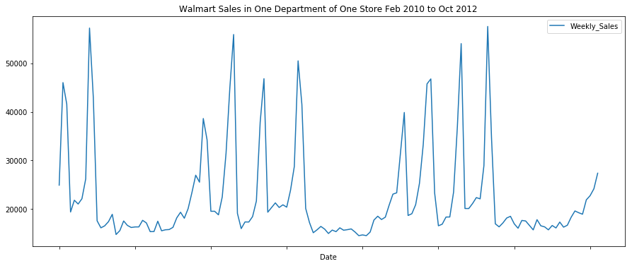
We can see that there are some clear patterns in the data. Through simple eye-balling, there are four spikes in sales around November, December, February, and April.
dat.index = pd.to_datetime(dat.index)
from statsmodels.tsa.seasonal import seasonal_decompose
result = seasonal_decompose(dat, model='multiplicative')
fig = result.plot()
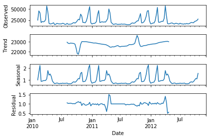
From the plot above we can clearly see the seasonal component of the data, and we can also see the separated bumpy trend of the data.
Forecast Model
Now let’s build an ARIMA model to predict sales over time. ARIMA (autoregressive integrated moving average) models, also called Box-Jenkins models, are a class of powerful and popular models to forecast time series data. The ARIMA models may possibly include autoregressive terms, moving average terms, and differencing operations.
AR: Autoregression. A model that uses the dependent relationship between an observation and some number of lagged observations. AR(1): a linear model to predict the value at the present time using the value at the previous time.
I: Integrated. The use of differencing of raw observations (e.g. subtracting an observation from an observation at the previous time step) in order to make the time series stationary.
MA: Moving Average. A model that uses the dependency between an observation and a residual error from a moving average model applied to lagged observations.
ARIMA models are commonly denoted as ARIMA(p,d,q) where the parameters are substituted with integer values to quickly indicate the specific ARIMA model being used. A value of 0 can be used for a parameter, which indicates to not use that element of the model. This way, the ARIMA model can be configured to perform the function of an ARMA model, and even a simple AR, I, or MA model.
from pyramid.arima import auto_arima
stepwise_model = auto_arima(dat, start_p=1, d=1, start_q=1,
                           max_p=3, max_q=3, m=12,
                           start_P=0, seasonal=True,
                           D=1, trace=True,
                           error_action='ignore',
                           suppress_warnings=True)
print(stepwise_model.aic())
Fit ARIMA: order=(1, 1, 1) seasonal_order=(0, 1, 1, 12); AIC=2760.510, BIC=2774.848, Fit time=1.505 seconds
Fit ARIMA: order=(0, 1, 0) seasonal_order=(0, 1, 0, 12); AIC=2842.204, BIC=2847.939, Fit time=0.048 seconds
Fit ARIMA: order=(1, 1, 0) seasonal_order=(1, 1, 0, 12); AIC=2806.564, BIC=2818.034, Fit time=0.202 seconds
Fit ARIMA: order=(0, 1, 1) seasonal_order=(0, 1, 1, 12); AIC=2759.891, BIC=2771.361, Fit time=1.477 seconds
Fit ARIMA: order=(0, 1, 1) seasonal_order=(1, 1, 1, 12); AIC=2789.475, BIC=2803.813, Fit time=0.486 seconds
Fit ARIMA: order=(0, 1, 1) seasonal_order=(0, 1, 0, 12); AIC=2842.065, BIC=2850.668, Fit time=0.145 seconds
Fit ARIMA: order=(0, 1, 1) seasonal_order=(0, 1, 2, 12); AIC=nan, BIC=nan, Fit time=nan seconds
Fit ARIMA: order=(0, 1, 1) seasonal_order=(1, 1, 2, 12); AIC=2784.482, BIC=2801.687, Fit time=12.198 seconds
Fit ARIMA: order=(0, 1, 0) seasonal_order=(0, 1, 1, 12); AIC=2758.284, BIC=2766.887, Fit time=0.798 seconds
Fit ARIMA: order=(0, 1, 0) seasonal_order=(1, 1, 1, 12); AIC=2760.066, BIC=2771.537, Fit time=1.015 seconds
Fit ARIMA: order=(0, 1, 0) seasonal_order=(0, 1, 2, 12); AIC=nan, BIC=nan, Fit time=nan seconds
Fit ARIMA: order=(0, 1, 0) seasonal_order=(1, 1, 2, 12); AIC=2790.007, BIC=2804.345, Fit time=4.098 seconds
Fit ARIMA: order=(1, 1, 0) seasonal_order=(0, 1, 1, 12); AIC=2760.133, BIC=2771.603, Fit time=1.594 seconds
Total fit time: 23.614 seconds
2758.2843325496183
Now we can pick the model with the best performance and validate the model performance by splitting the data into a train and a test set.
train = dat.loc[:'2012-05-01']
test = dat.loc['2012-05-01':]
stepwise_model.fit(train)
ARIMA(callback=None, disp=0, maxiter=50, method=None, order=(0, 1, 0),
   out_of_sample_size=0, scoring='mse', scoring_args={},
   seasonal_order=(0, 1, 1, 12), solver='lbfgs', start_params=None,
   suppress_warnings=True, transparams=True, trend='c')
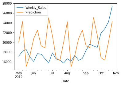
future_forecast = stepwise_model.predict(n_periods=len(test))
future_forecast = pd.DataFrame(future_forecast,index = test.index,columns=['Prediction'])
pd.concat([test,future_forecast],axis=1).plot()
<matplotlib.axes._subplots.AxesSubplot at 0x7f4ffc078490>
pd.concat([dat,future_forecast],axis=1).plot(figsize=(15, 6),
                                             title="Walmart Sales in One Department of One Store Feb 2010 to Oct 2012")
<matplotlib.axes._subplots.AxesSubplot at 0x7f4fd2f3c0d0>
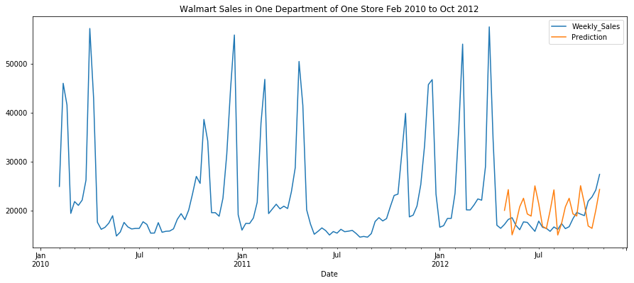
Conclusion
Voilà! Now we have a forecast model that can predict the sales of the coming weeks. With real-world data, the predictions will almost never be 100% in sync with the data, but we can see that the predictions stay in a reasonable range for off-holiday season sales. We can use the forecast information to optimize staffing and other resources.